Statistics and SimulationsJanuary 1, 2019

Introduction

Stochastic simulation, also commonly known as "Monte Carlo" simulation, generally refers to the use of random number generators to model chance/probabilities or to simulate the likely effects of randomly occurring events. A random number generator is any process that produces data whose observations are independent and identically distributed (i.i.d), from a distribution. Stochastic modeling utilizes the random aspects of the generated data to evaluate processes or systems using probabilities based on repeatedly sampling from the randomly generated numbers. With the rapid increase (and the concurrent decrease in cost) of computing power, the use of stochastic simulation has played an increasingly large role in statistics. Stochastic simulations can be used to model complicated processes and to estimate distributions of estimators (using methods such as bootstrap). Stochastic simulations also have dramatically increased the use of an entire field of statistics, Bayesian statistics, because simulation can be used to estimate the distribution of its statistics, which are usually analytically intractable except in the simplest situations. This paper provides an introductory explanation of Monte Carlo simulation in the context of process modeling, and the benefits of using this analytical technique as a tool for process improvement.

Monte Carlo analysis can be employed wherever a transfer function is used to express the relationship between independent and dependent variables: processes, physical equations, mathematical relationships, etc. In the context of process improvement, Monte Carlo analysis can be useful when assessing the impact of variation on a process. Often processes are mapped and analyzed in a static manner. But real‐world conditions typically involve variation. Monte Carlo simulation introduces variation into a process model such that the effects of variation on the process can be observed. Specifically, stochastic modeling helps assess how variation in the independent process variables (inputs) produces effects on the dependent variable (output) for systems that are both discrete and stochastic. The primary purpose of such modeling is to identify which independent variables have the highest correlation with the dependent variable and use that relationship as a basis for improvement or optimization efforts.

Simulation by random sampling was in use during the genesis of probability theory, long before computers. Toss a coin a hundred times and count the number of times it falls "heads." Dividing the total number of times the coin falls heads by the total number of tosses gives the basis for estimating the probability of heads for that coin, using simulation. The error associated with that estimate is called "Monte Carlo error."

Stochastic simulation was used as far back as in 1777 by Buffon to estimate the probability of a needle falling across a line in a uniform grid of parallel lines, a study known as "Buffon's needle problem." William Gosset, who derived the t-distribution, also used stochastic simulation techniques in the early 1900s for his work on small samples. The name "Monte Carlo Simulation" was coined in the 1940s by a group of scientists working on the Manhattan Project at Los Alamos National Laboratory. That group used simulation to calculate the probability with which a neutron from the fission of one uranium atom would cause another atom to fission. The method was named after the casino in Monte Carlo, Monaco, and refers to the fact that gambling chances are based on randomness and repetitive sampling, as is Monte Carlo simulation.

With the advent of computers, the availability and use of random number generators have increased so that they are now easily obtained and can be customized for particular uses and distributions. For example, Microsoft Excel can generate random numbers from many standard distributions, such as Uniform, Normal, Binomial, etc. The random number generator is available under the Data Analysis function in the Tools menu in Excel.

An Example of Monte Carlo Simulation

Here's an example of how Monte Carlo simulation can be used to assess and minimize wait time at a restaurant drive‐through window. In this illustrative case, for which we will use EngineRoom data analysis software, a national fast food chain wanted to reduce the amount of time customers spend in the drive‐through by limiting their wait to under three minutes at least 90% of the time. The response/dependent variable of the process is the lag between the time the customer completes their order and the time the customer picks up the order (the "Drive‐Through Cycle Time"). The Drive‐Through Cycle Time has four individual components/process steps: Prepare, Cook, Package, and Deliver. The drive‐through cycle time (TDrive‐through) is modeled as the sum of the cycle times of each of the individual steps:

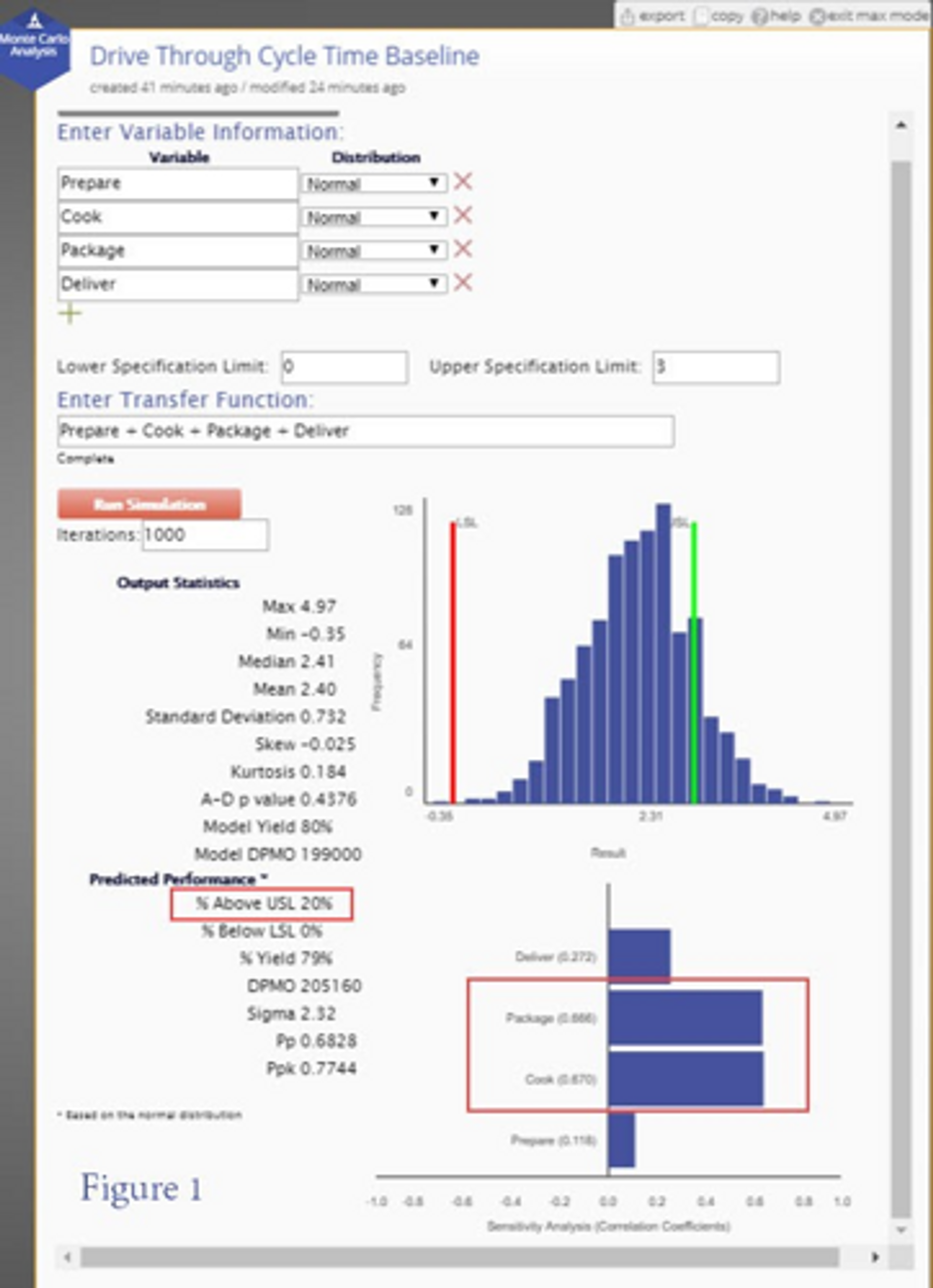
Using historical data, the underlying distributions for the individual process steps were found to be normal. The normal distribution parameters (means and variances) and the specification for Tdrive‐through (upper specification = 3 minutes) were entered into the Monte Carlo analysis tool provided by EngineRoom. The simulation was run 1,000 times using randomly generated values for each independent variable according to the distributions defined for each, yielding the histogram shown in Figure 1.

The green vertical line represents the upper specification of 3 minutes. In the current process only 80% of the wait times are below 3 minutes. The modeling results also include a sensitivity analysis showing that the process steps of packaging and cooking are equally large contributors to the variation in the cycle time response.

Further analysis was done on the packaging and cooking processes. One option considered was to use pre‐cooked rather than cooked-to-order burgers. Doing so would drastically reduce the wait time, and that model showed that the improved process would consistently produce wait times under 3 minutes 99.4% of the time. But that option entailed possible costs in terms of customer satisfaction by modifying the product, possibly contrary to market expectations, and in terms of unusable inventory/spoilage. For those reasons, and because packaging and cooking were comparable factors for process sensitivity, the team decided to reduce the mean time and variation experienced in packaging the cooked food.

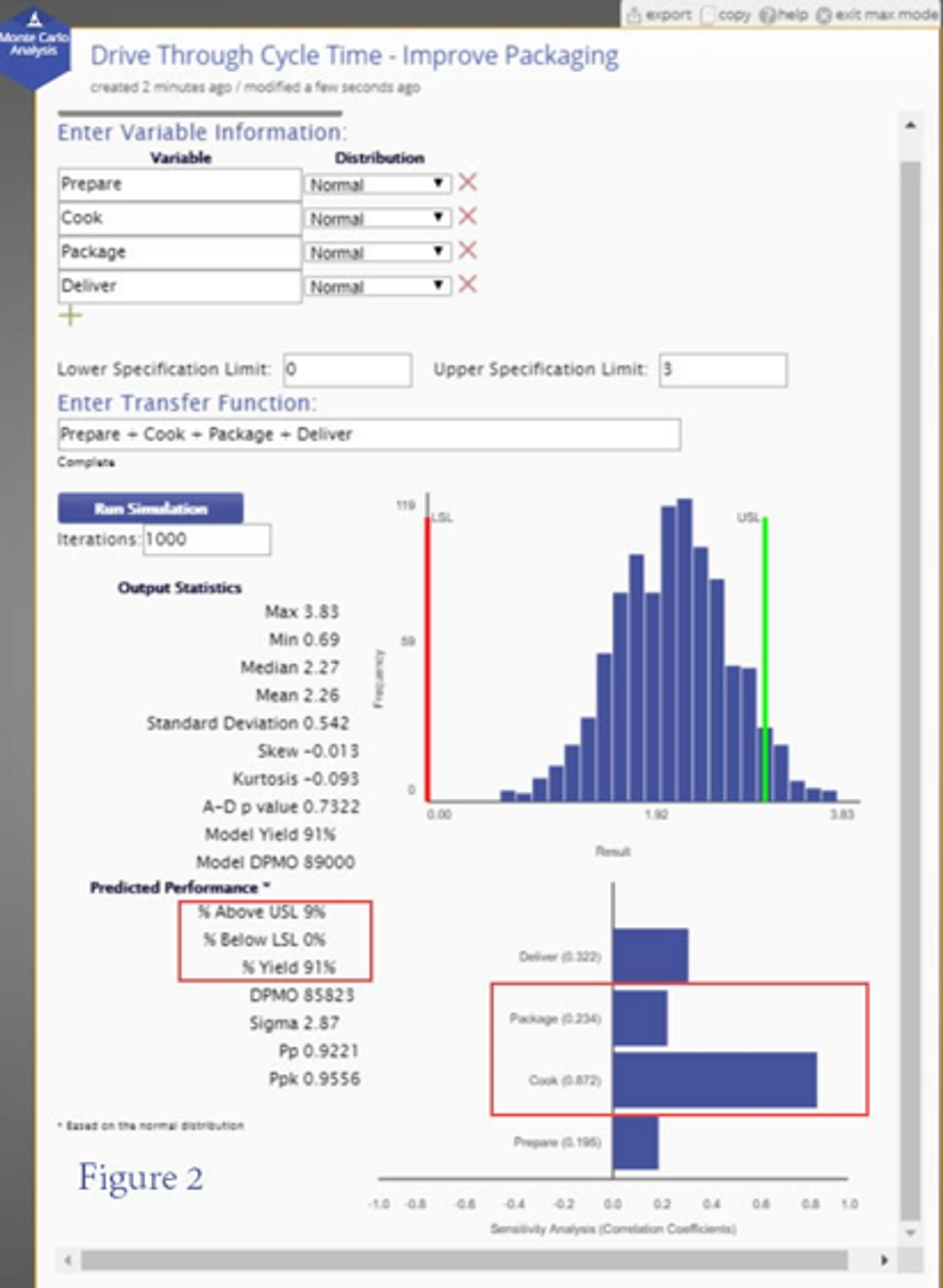
The packaging improvement team determined that multiple package designs with differing cartons and wrappers, lid sizes and individual utensils created both, a higher than necessary mean process time, and excessive variation. By pre-positioning packaging materials, implementing common packages and sizes, and removing rarely used packaging items, the team estimated it could achieve the required efficiencies without affecting the food or the customer's eating experience. Based on a prototype set-up, the team estimated new process parameters for the improved packaging process. The histogram for the new, improved process is shown in Figure 2.

With the new packaging process, the distribution of the overall dependent variable (Tdrive‐through) shifted to the left and tightened such that 91% of the traffic would wait less than the 3‐minute tolerance, with any wait times of 4 minutes or over likely to be rare. This expected level of performance met the stated business objective of 90% of drive through traffic experiencing a wait time of 3 minutes or less. On that basis, the team decided to implement the improved process through a pilot program so that the process parameters used in the model could be validated by process data derived in the field.

Notably, and reflecting the changes made, the sensitivity of the overall process to variation in the packaging sub‐process was greatly reduced. Any further improvements in Drive‐Through Cycle Time would likely have to entail consideration of the cooking processes rather than further improvement in packaging.

Summary

This was a simple demonstration of Monte Carlo simulation, to give you an idea of how to use this tool. A primary benefit of this method is that an improvement can be evaluated without disrupting the actual process. Different scenarios can thus be compared, and the one resulting in the best results applied to the production process. At the same time, a few things to keep in mind are:

1. Assigning an incorrect distribution or parameters to an input will lead to incorrect predictions.
2. The method assumes that the inputs are independent ‐ this may not be valid.

Still, these are minor drawbacks in a method that is amazingly versatile and powerful for assessing uncertainty in the output of complex stochastic models.