Response Optimizer Tutorial
Table of Contents
Single Output: Using a Regression or DOE Tool
Single Output: Building Your Own Equation
Multiple Outputs: Using Regression Tools
Multiple Outputs: Using DOE Tools
Multiple Outputs: Building Your Own Equation
Cost
Weights
Tutorial
Coming Soon
When to use this tool
Use the Response Optimizer to calculate the response of an equation and determine the values of the inputs that maximize, minimize, or hit a target for the response. This tool is best paired with Regression tools that calculate an equation and then using the Optimizer to optimize the value of that response.
The Response Optimizer is also able to handle multiple equations with shared input factors. You can optimize up to three equations simultaneously* as well as a fourth Cost variable.
*All outputs have equal weight in the output. At this time, there is no method for indicating one equation is more important to hit its target than another.
Using EngineRoom
Single Output: Using a Regression or DOE tool
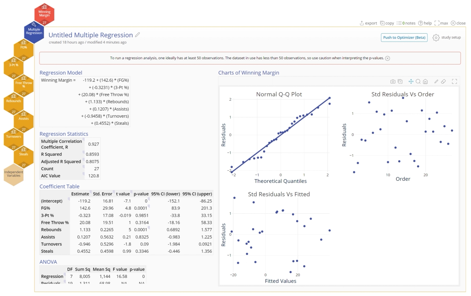
1. Complete a Multiple Regression tool or a DOE tool in EngineRoom.
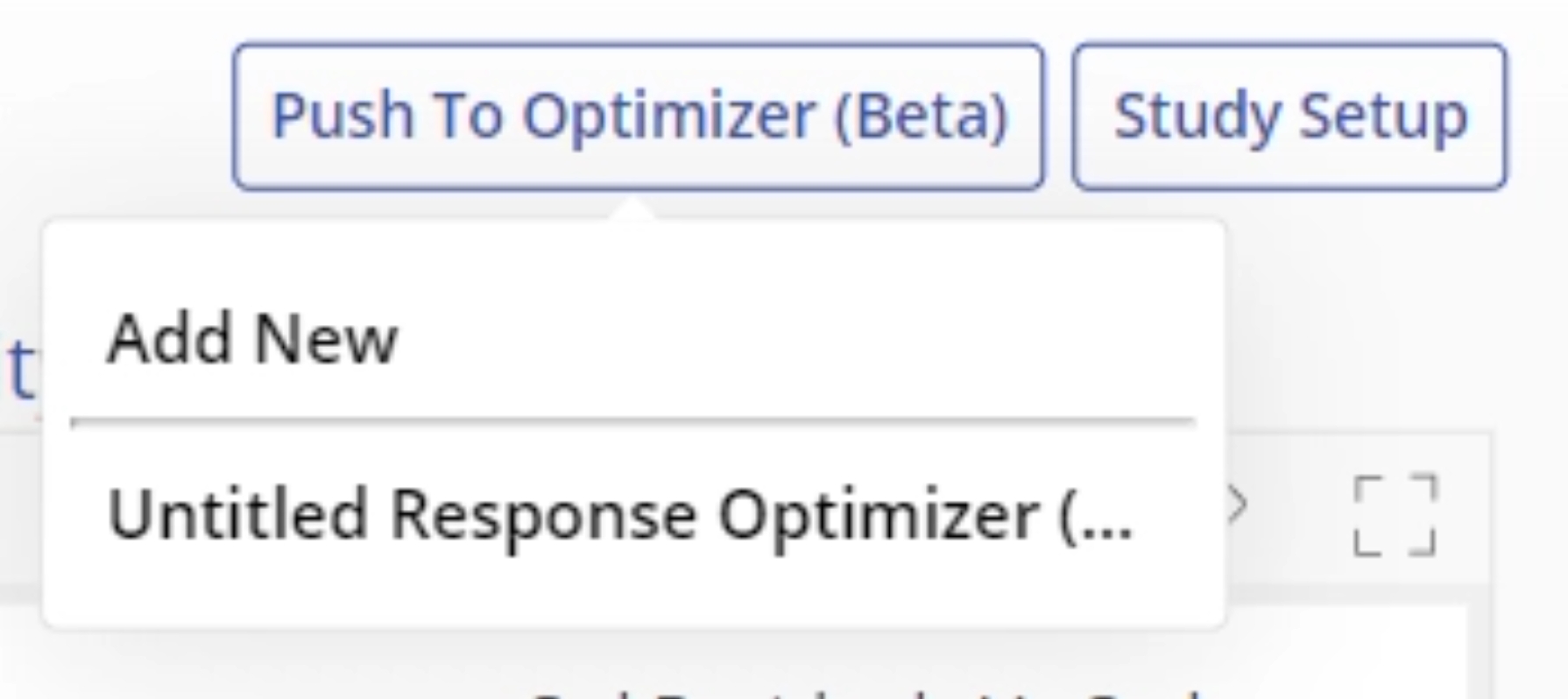
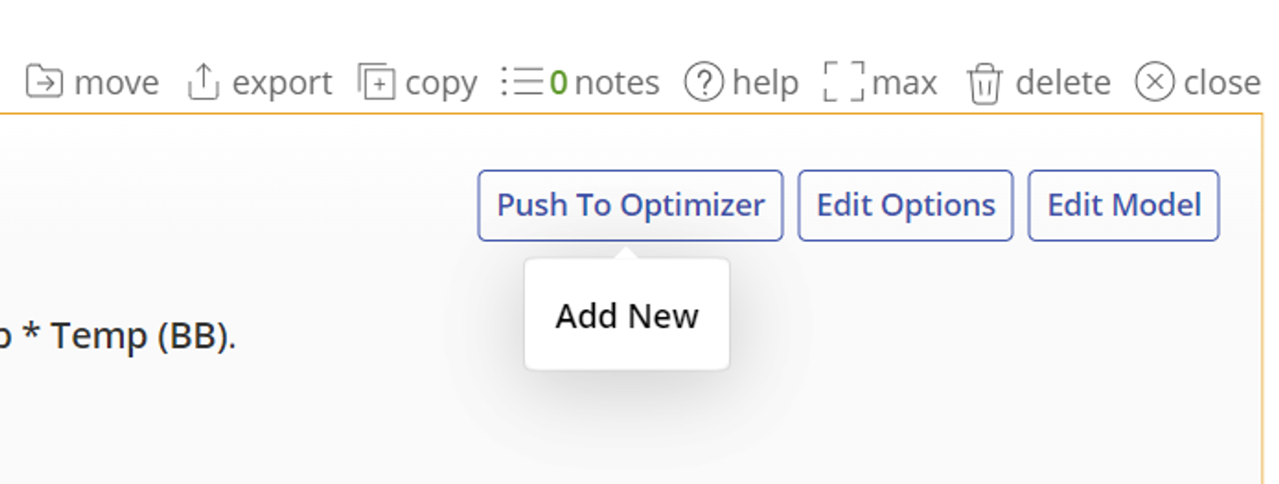
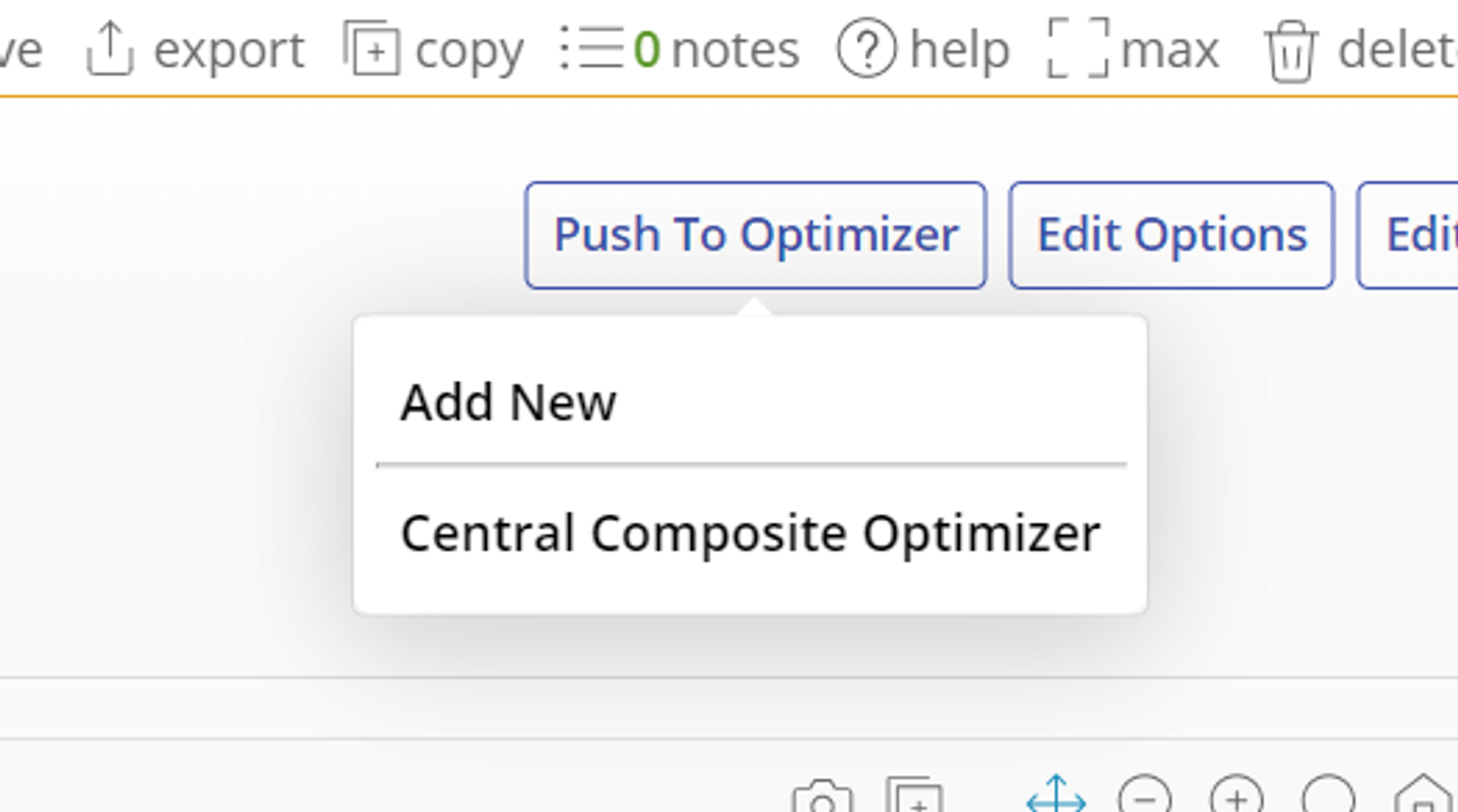
2. Once you get to the results screen, click the "Push to Optimizer" button on the top right corner of the study and then click "Add New".
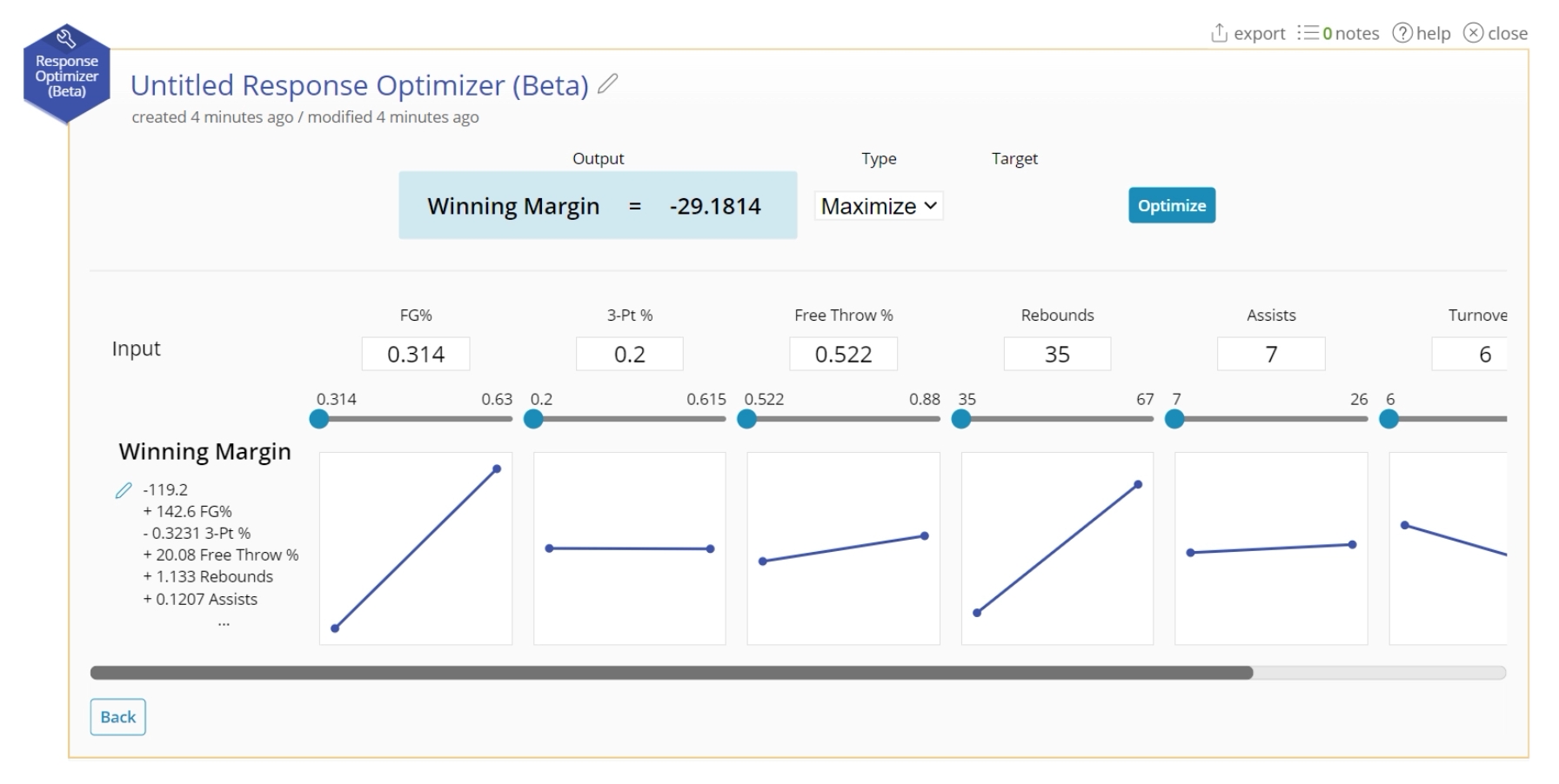
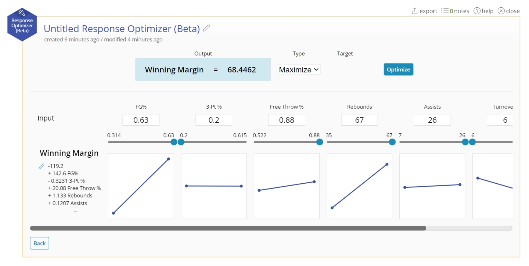
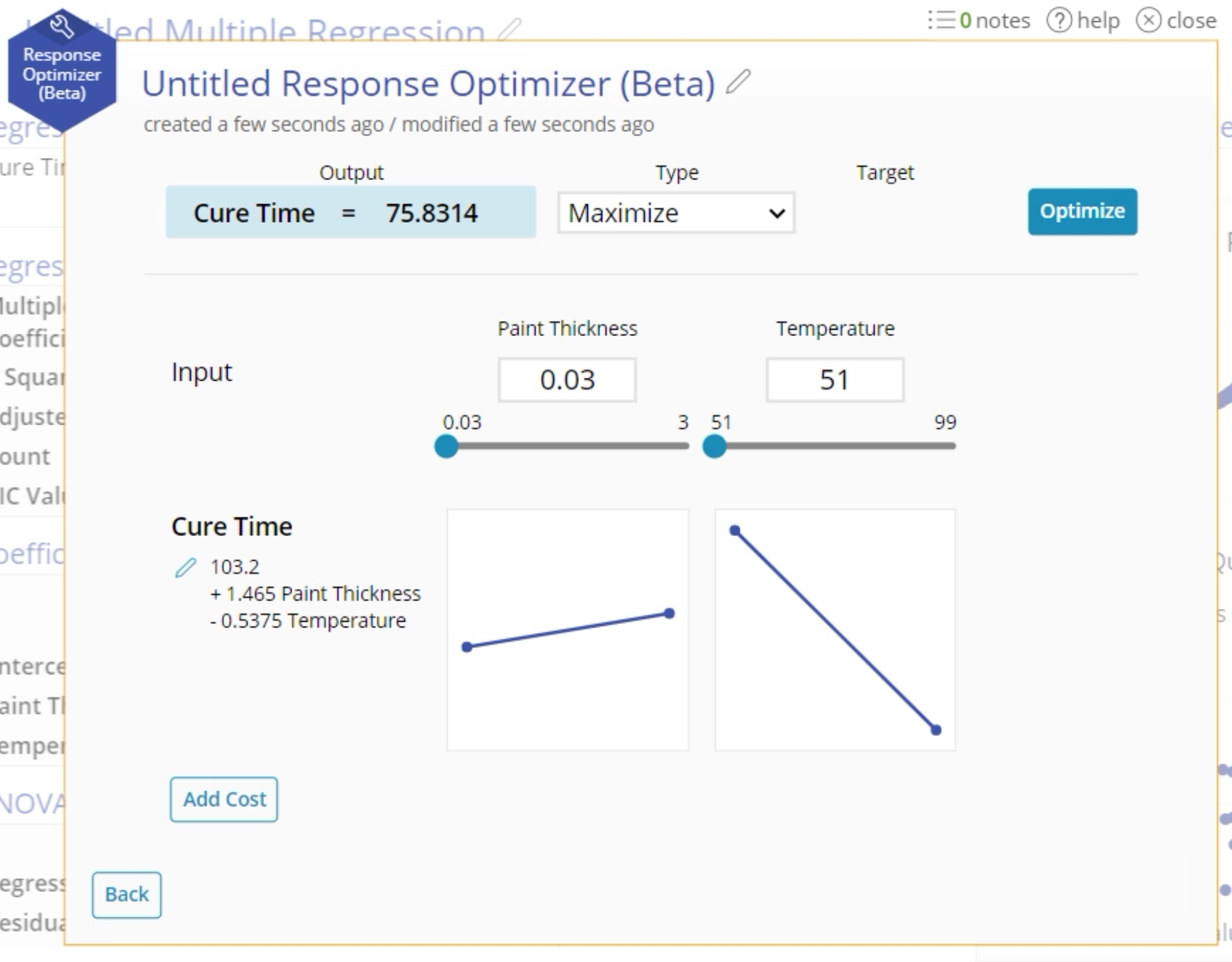
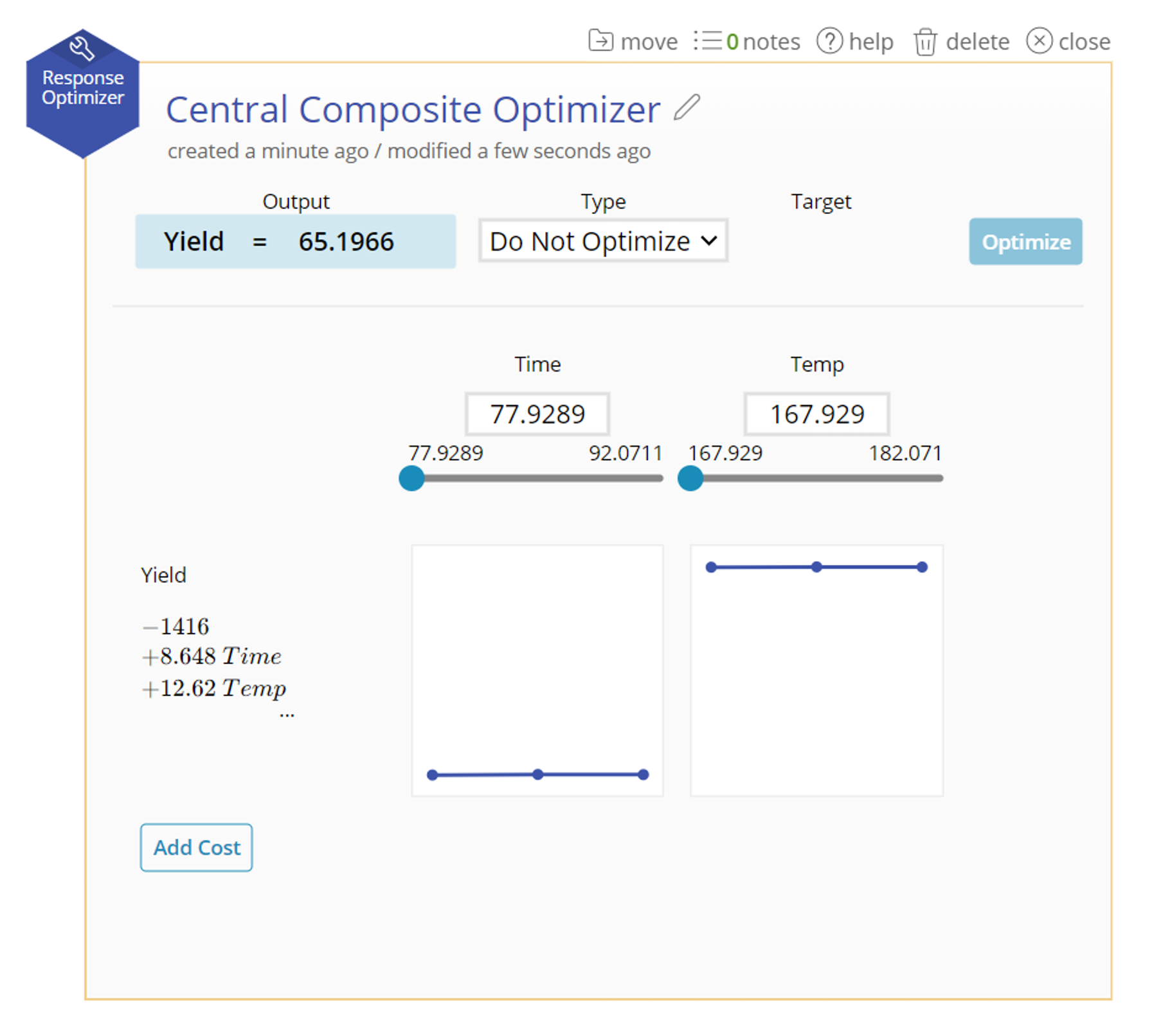
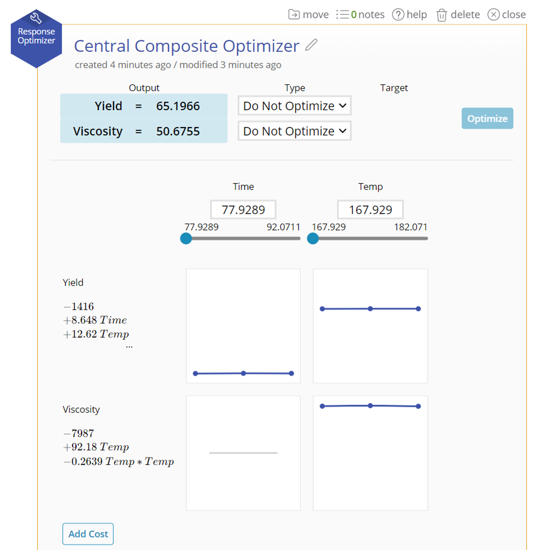
3. The Optimizer will open with your equation. The output will be set based on the minimum value of your input variables.
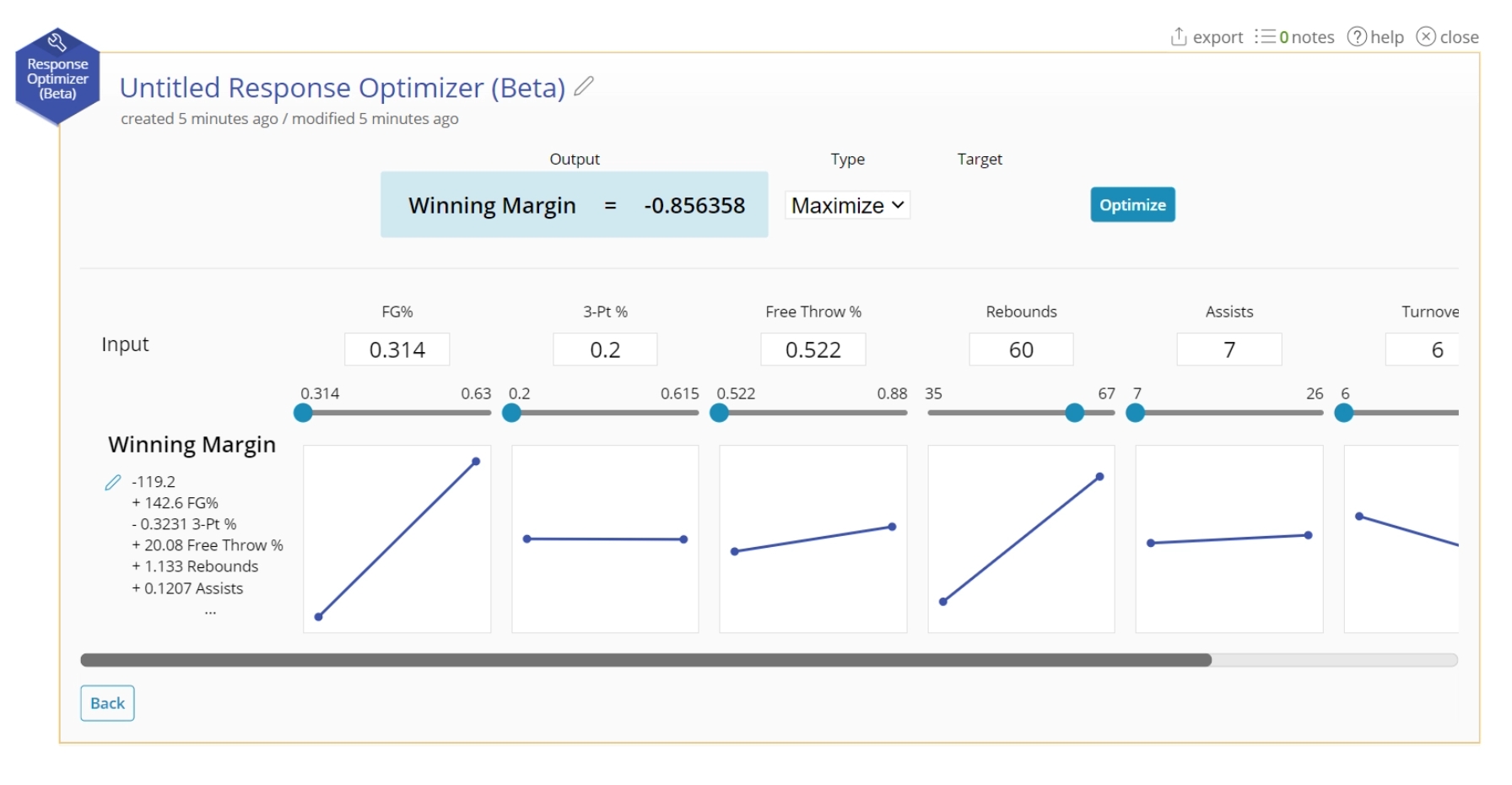
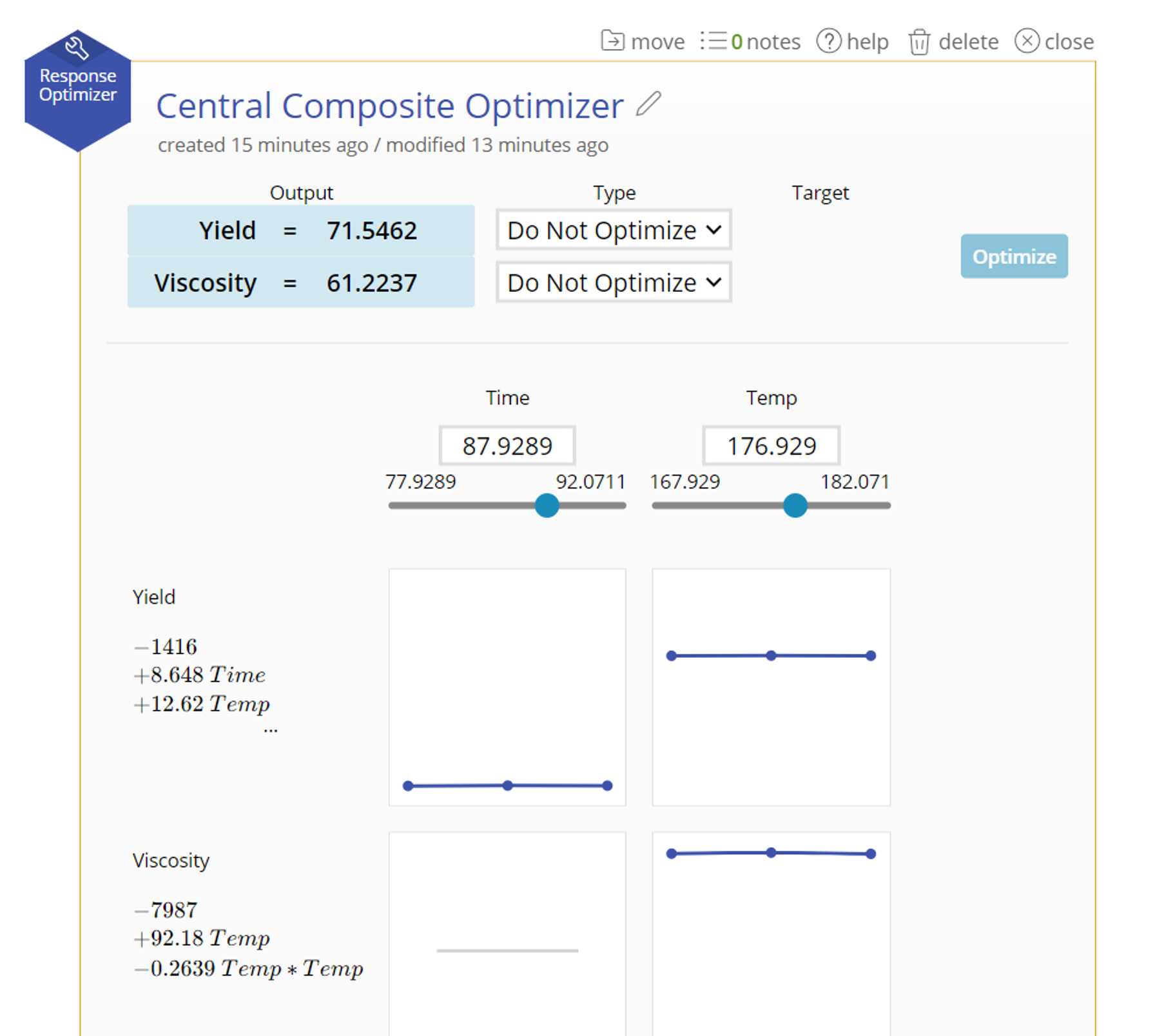
4. Manually calculate the resulting output from a series of inputs by using the text box to set a value, or sliding with the slider.
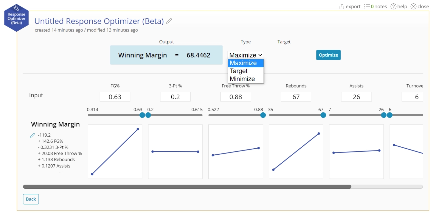
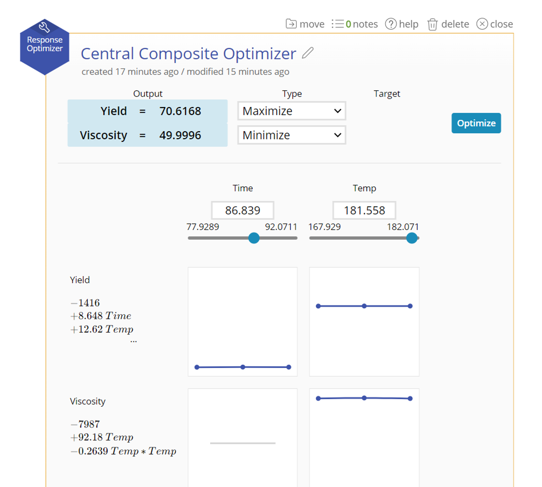
5. For your response, select "Maximum", "Minimum", or "Target". If you select "Target", type in a value to attempt to hit.
6. Click "Optimize".
7. The optimal value will display in the blue box. The corresponding input variables will change to fit in those spaces.
Single Output: Building Your Own Equation
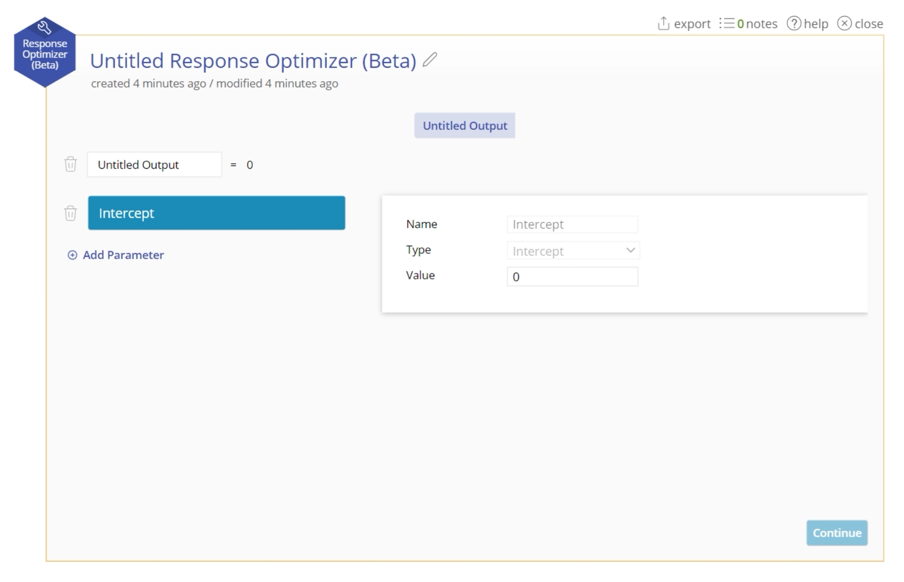
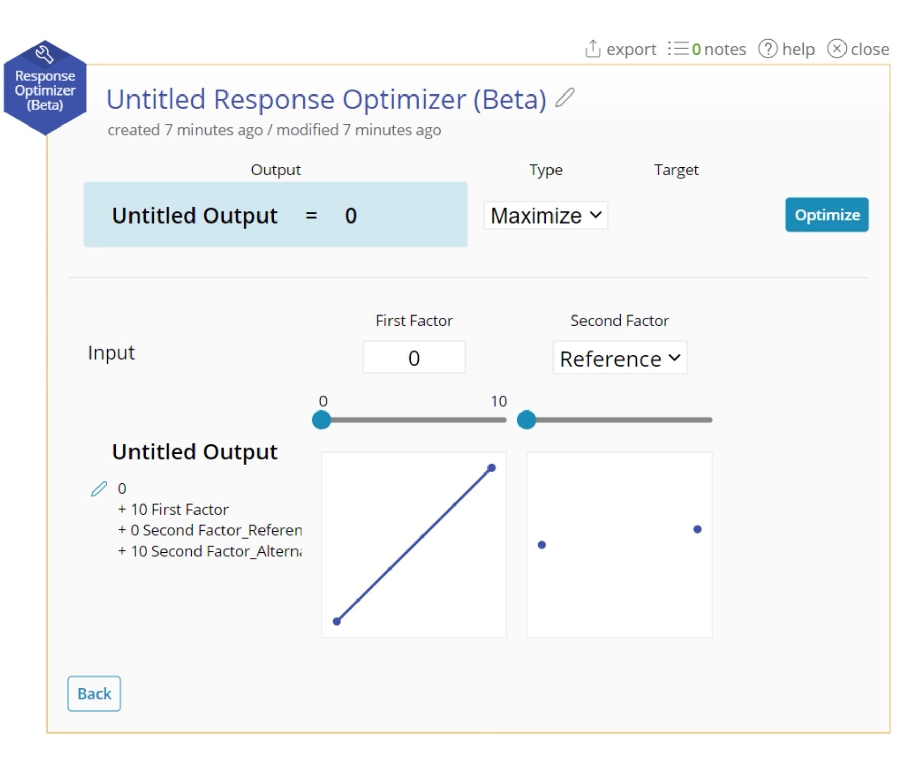
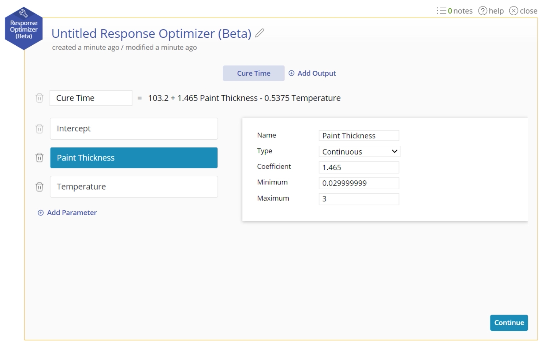
1. Open a new Response Optimizer from the tools menu. A new equation screen will appear to allow you to build your equation.
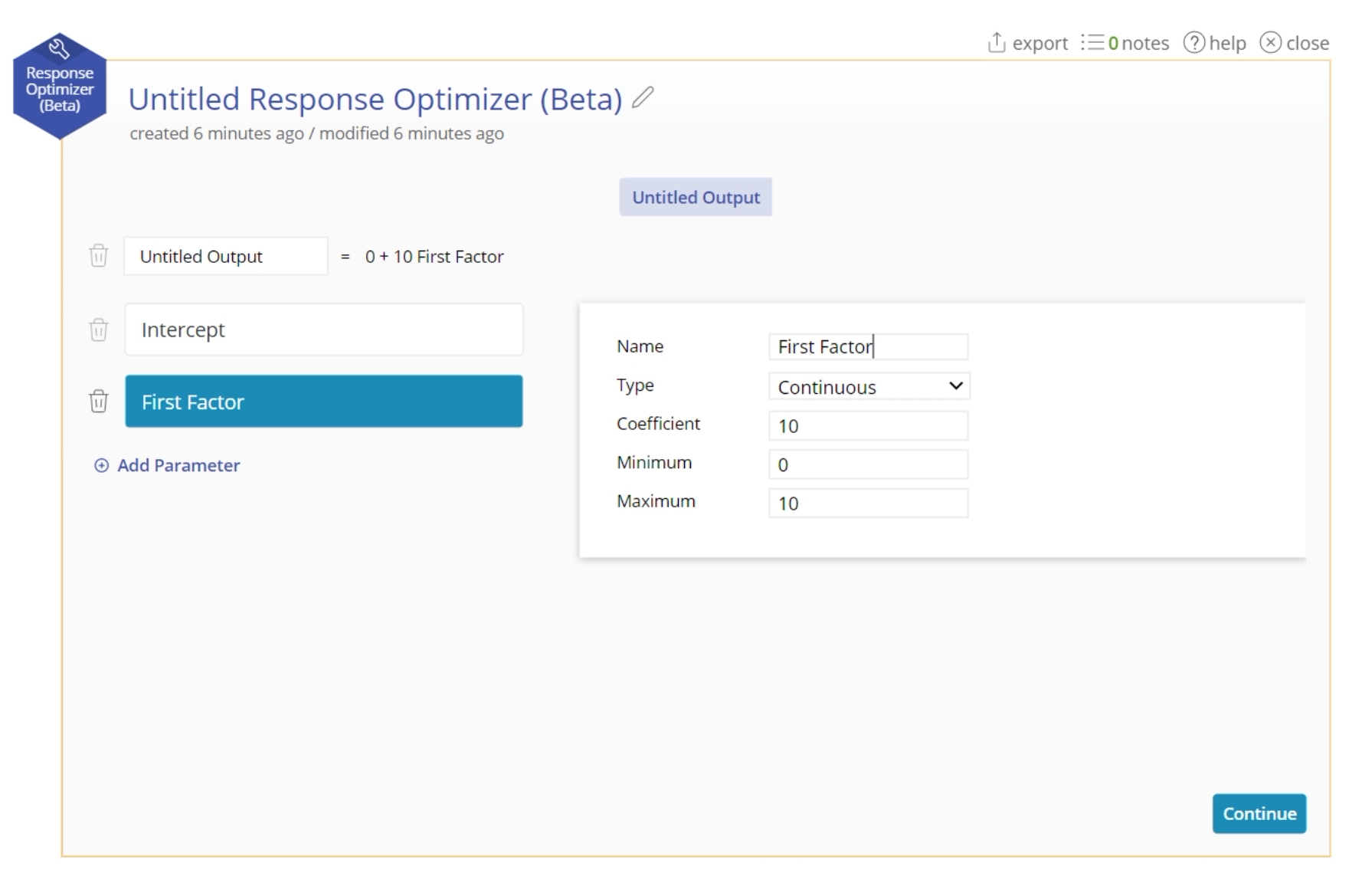
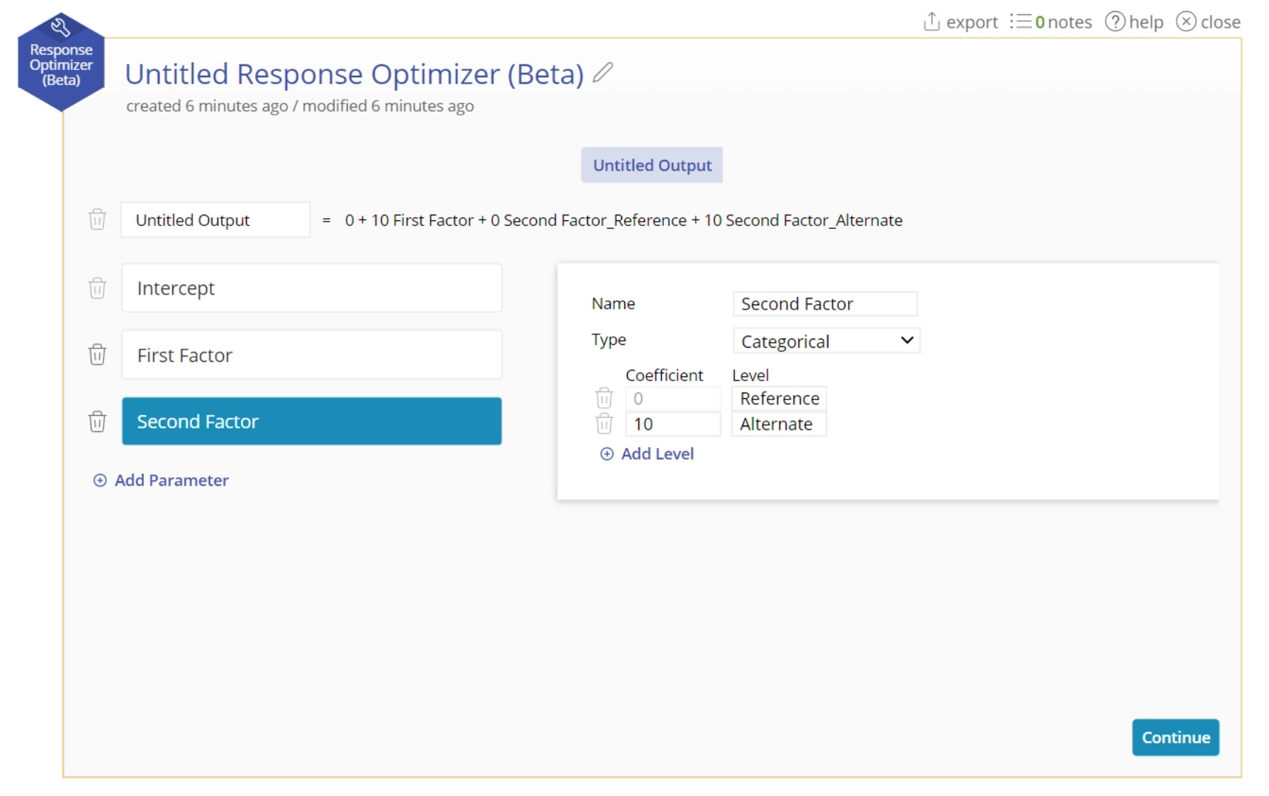
2. Add each factor in your equation along with its coefficient:
- Intercept: This is the y-intercept of your equation. If all of your factors were set to 0, what would the equation equal?
- Continuous: A continuous numeric factor. You must set the minimum, maximum, and decimal spaces in order to set the parameter space for optimization.
- Categorical: A categorical factor that contains 2 or more levels. The first level is the reference level, the one on which every other level's coeffcient is based. There is only 1 level active at a time in the equation.
3. Building out your equation this way ensures that you will have all the information necessary for doing your optimization.
4. Click "Continue".
5. The interface now allows you to manipulate the inputs to get the related output response.
Multiple Outputs: Using Regression Tools
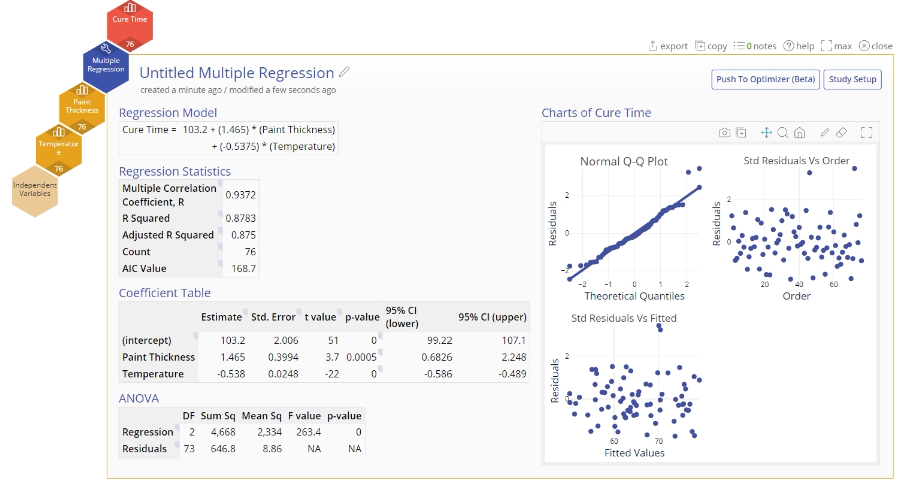
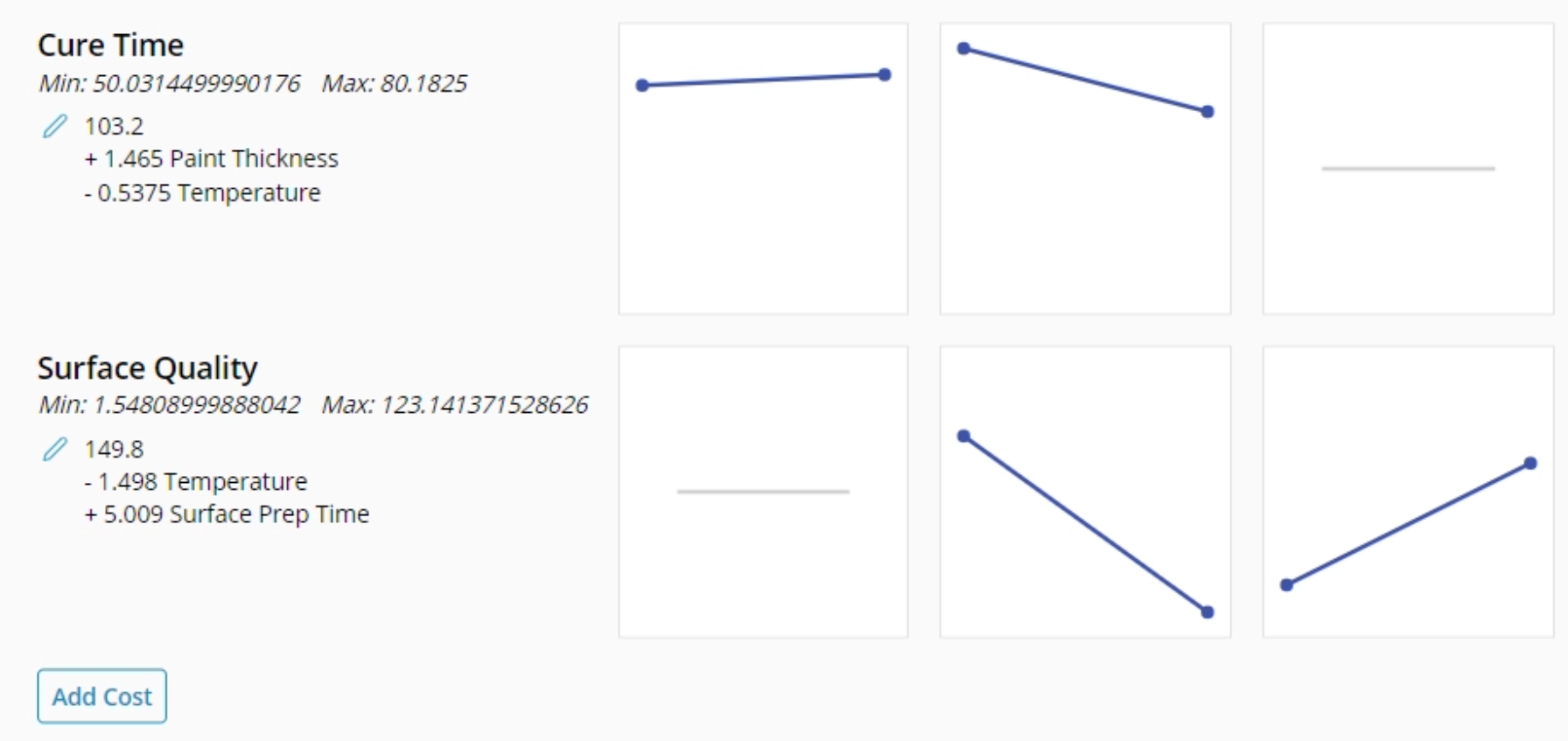
A manufacturing company wants to minimize the Cure Time and maximize the Surface Quality score. The Cure Time equation includes Paint Thickness and Temperature, while the Surface Quality equation includes Temperature and Surface Prep Time. Download the data above to complete this example.
1. Complete a Multiple Regression tool in EngineRoom. For this example, use the Paint Thickness and Temperature as input variables and Cure Time as the output variable.
2. Once you get to the results screen, look for the "Push to Optimizer" button on the top right corner of the study. Click the "Push to Optimizer" button, and select "Add New".
3. The Optimizer will open with your equation. The output will be set based on the minimum value of your input variables.
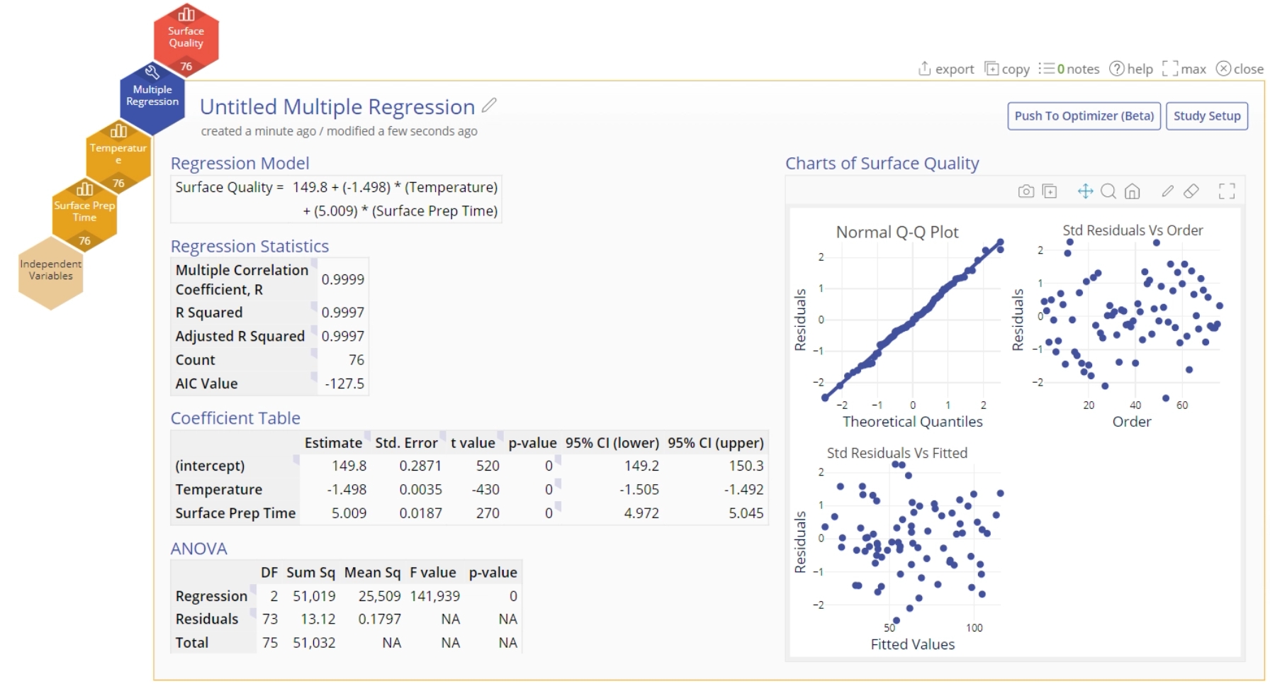
4. Create a second Multiple Regression tool. For this example, use the Temperature and Surface Prep Time as input variables and Surface Quality as the output variable.
5. Once you get to the results screen, click the "Push to Optimizer" button and select the existing Optimizer.
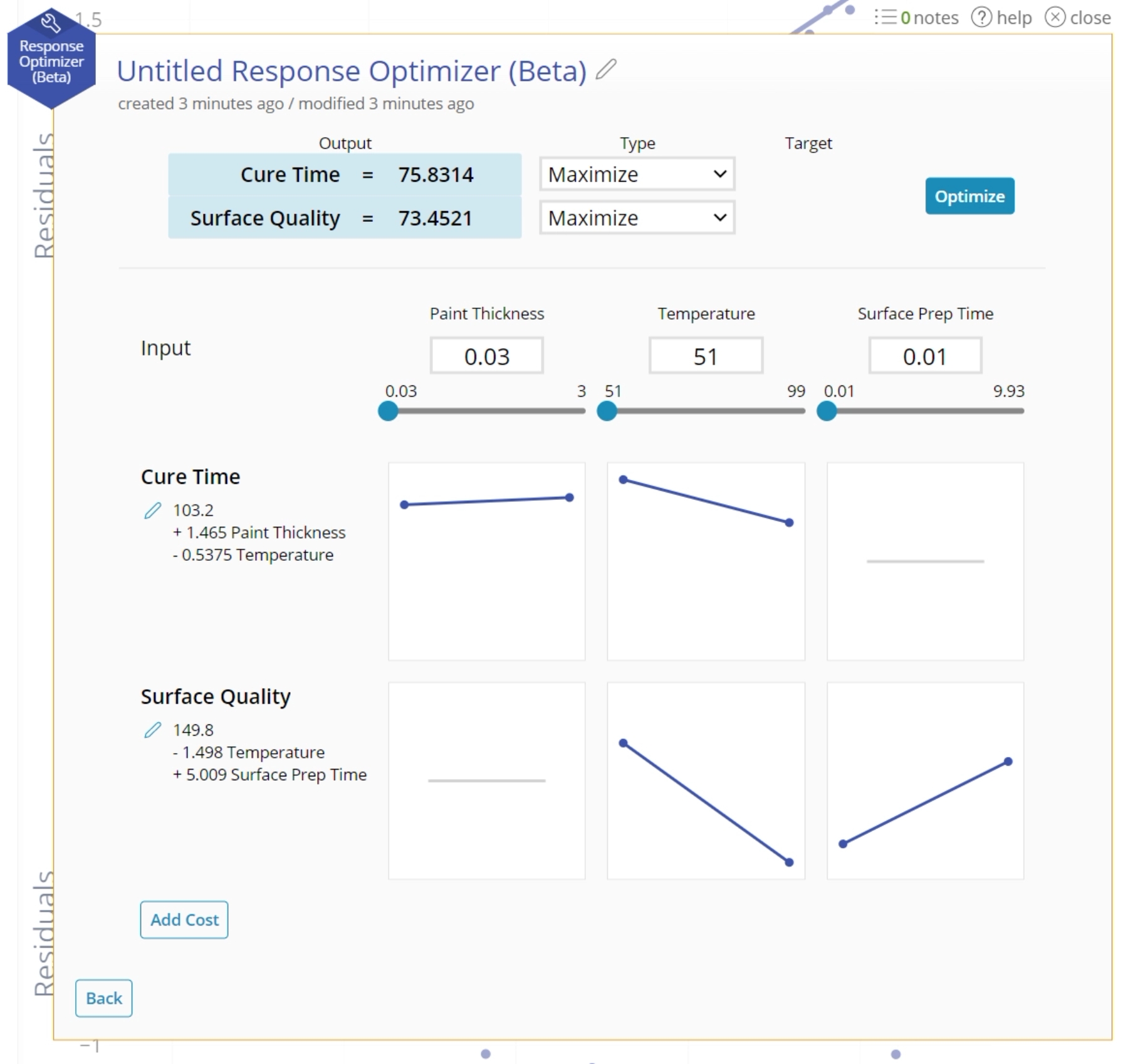
6. The second equation will be added to the Optimizer tool allowing you to manipulate the values of both at the same time. Note: because the input factor "Temperature" has the same name in both cases, the factor is shared between the two outputs and controls the calculation of both.
7. Manually calculate the resulting output from a series of inputs by using the text box to set a value, or sliding with the slider. The shared factors will recalculate both equations, while factors for just one equation will just recalculate the one output.
8. For each of your responses, select "Maximum", "Minimum", or "Target". If you select "Target", type in a value to attempt to hit. For our example, we'll set Cure Time to Minimum and Surface Quality to Maximum.
9. Click "Optimize".
10. The optimal values will display in the blue box. The corresponding input variables will change to fit in those spaces. Note: The equations are treated with equal weight. Therefore, it might not completely maximize or minimize a particular output but will find the best for both. See Weights at the bottom of this article.
Multiple Outputs: Using DOE Tools
1. Complete a DOE tool in EngineRoom. This can be Full Factorial, Fractional Factorial, General Factorial, or Response Surface Methodology.
2. Once you get to the results screen, look for the "Push to Optimizer" button on the top right corner of the study. Click the "Push to Optimizer" button, and select "Add New".
3. The Optimizer will open with your equation. The output will be set based on the minimum value of your input variables.
4. Create a second DOE tool. Usually this will involve dragging on your existing DOE Matrix with a different Response Variable.
5. Once you get to the results screen, click the "Push to Optimizer" button and select the existing Optimizer.
6. The second equation will be added to the Optimizer tool allowing you to manipulate the values of both at the same time. Note: Factor with the same name is shared between the two outputs and controls the calculation of both.
7. Manually calculate the resulting output from a series of inputs by using the text box to set a value, or sliding with the slider. The shared factors will recalculate both equations, while factors for just one equation will just recalculate the one output.
8. For each of your responses, select "Maximum", "Minimum", or "Target". If you select "Target", type in a value to attempt to hit.
9. Click "Optimize".
10. The optimal values will display in the blue box. The corresponding input variables will change to fit in those spaces. Note: The equations are treated with equal weight. Therefore, it might not completely maximize or minimize a particular output but will find the best for both. See Weights at the bottom of this article.
Multiple Outputs: Building Your Own Equation
1. Open a new Response Optimizer from the tools menu. A new equation screen will appear to allow you to build your equation.
2. Add each factor in your equation along with its coefficient. (Go to Factor Types to understand what they mean). Building out your equation this way ensures that you will have all the information necessary for doing your optimization.
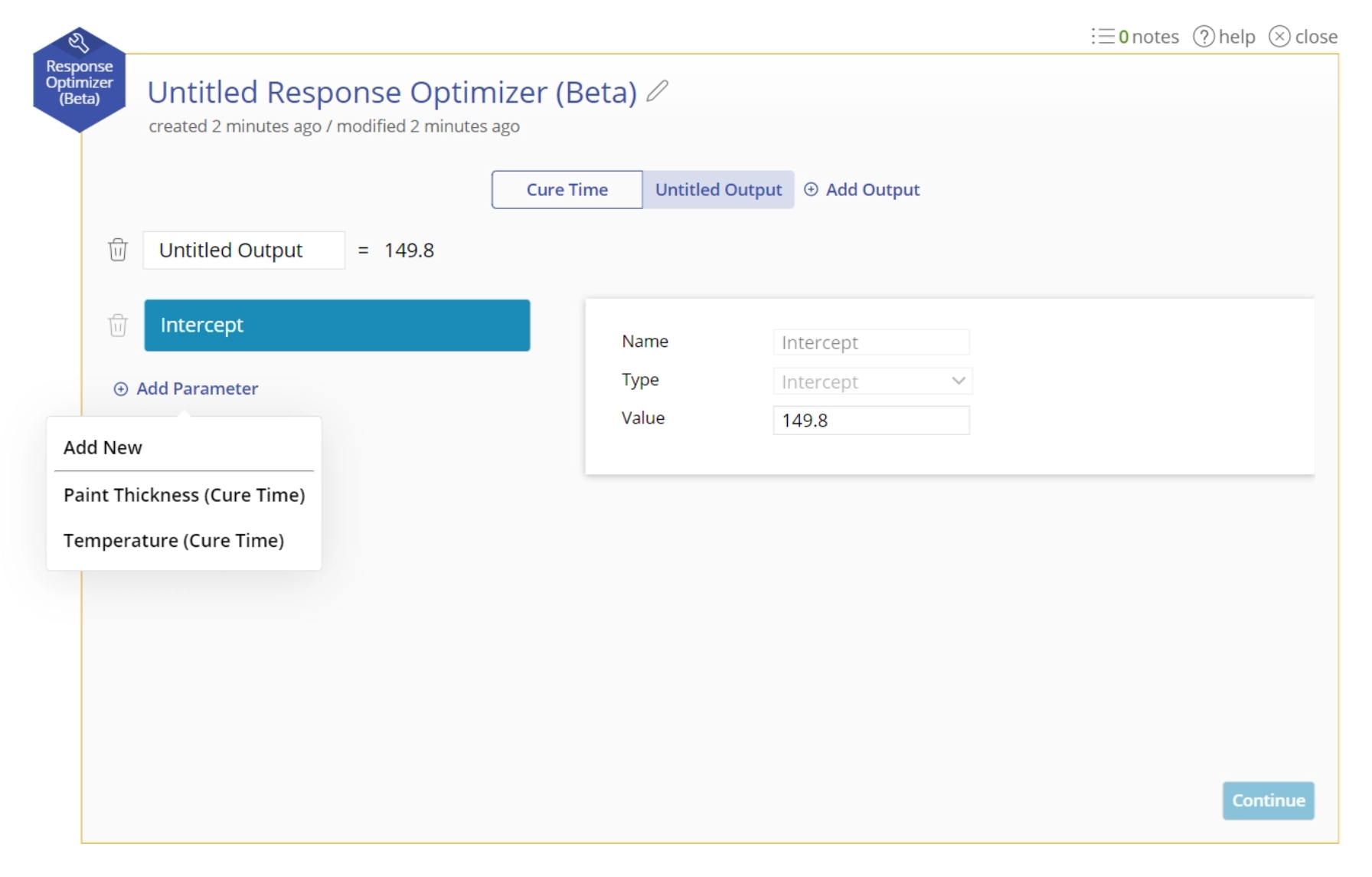
3. Click "Add Output". Now you can build a second equation. You can have a total of 3 equations.
4. Build your second equation by add each factor in your equation along with its coefficient. (Go to Factor Types to understand what they mean). When you click "Add Factor", you now have the option of adding factors that are shared between the equations.
- For Continuous Factors, the Maximum and Minimum will be shared between the two factors, but you can set unique coefficients for each equation.
- For Categorical Factors, the Levels will be consistent between the shared factors, but the coefficients for each level can change between the factors. If a level is not relevant to a function, just set its coefficient to 0.
5. When you are finished with your equations, click "Continue".
6. The interface now allows you to manipulate the inputs to get the related output responses.
Cost
1. Create an Optimizer. For this example, we completed the tutorial for Multiple Outputs: Using Regression Tools.
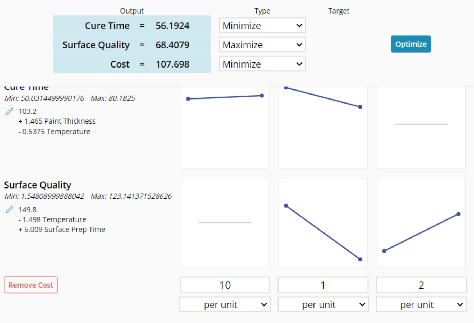
2. Click on the "Add Cost" button on the bottom left (you may need to scroll).
3. The Cost row will appear at the bottom and the Cost output will appear at the top.
4. Input your costs for each input factor.
- per unit: this option will multiply the number in the input field by the cost number. As you adjust the value of the input factor, the cost will be recalculated. For example, if the cost goes up $100 for each square foot, then you would put 100 in the cost, and as you adjust the square footage by 1, the cost will recalculate and add 100.
- fixed: this option will set a standard value to the cost that is not affected by the value of the input factor. For example, if it costs $300 because your car is painted regardless of the thickness of the paint, you can add 300 for fixed under Paint Thickness.
- Categorical Variables Only: by level: Each value under a categorical variable is able to have its own cost. For example, if you have a categorical Parking variable with levels No Parking, Covered Parking, or Individual Garage, you can set the price for each level. For example, select No Parking and set the price to $0, then select Covered Parking and set the price to $25, then select the Individual Garage Parking and set the price to $100. These prices will persist as you set the input factor level.
5. The cost will be calculated automatically at the top.
Weights
This tool can be used to optimize up to three responses simultaneously. To do this, the optimizer assigns each individual response a desirability function, ‘d’, which takes values ranging from 0 (least desirable) to 1 (most desirable) corresponding to the possible values of the response variable. The individual desirabilities are then combined using a composite desirability, D, which is basically the geometric mean of the individual desirabilities:
D = (d1* d2*…..*dk)1/k where di = the desirability of the ith response variable k = the number of responses being optimized.
Using the geometric mean ensures that the outcome is zero if any one response fails to achieve at least some measure of desirability.
When optimizing multiple equations at once:
- The optimizer treats each individual response as equally important. In other words, the importance score is equal for both responses. In the future, we would like to offer the ability to manipulate this score, setting a value ranging from 1 (least important) to 5 (most important).
- The optimizer places equal emphasis on the target and the bounds. In other words, the optimizer assigns all individual desirabilities a weight = 1. In the future, we would like to offer the ability to manipulate this weight assigned to the desirability function, which affects the shape of the desirability function.
Was this helpful?

